How To Make A Cashier Count Chart In Excel : Free Cashier Balance Sheet Template for Excel 2013 / Across the top row, (start with box a1), enter headings for the type of information you will enter into your run chart:

How To Make A Cashier Count Chart In Excel : Free Cashier Balance Sheet Template for Excel 2013 / Across the top row, (start with box a1), enter headings for the type of information you will enter into your run chart:. Enter the data you want to use to create a graph or chart. I am using ms office 2010. How to use the vlookup function in excel: Place charts neatly, one per cell. And, it's almost impossible to collaborate with stakeholders and team members.

On the insert tab click on the pivottable | pivot table (you can create it on the same worksheet or on a new sheet) on the pivottable field list drag country to row labels and count to values if excel doesn't automatically. Select your array of dates (with a header) and create a new pivot chart (insert / pivotchart / ok) then on the field list window, drag and drop the date column in the axis list first and then in the value list first. And, it's almost impossible to collaborate with stakeholders and team members. To generate a chart or graph in excel, you must first provide excel with data to pull from. The free cashier balance sheet template for excel 2013 is a template for keeping track of a cashier's daily financial transactions, ensuring that all the money adds up by the end of the day.

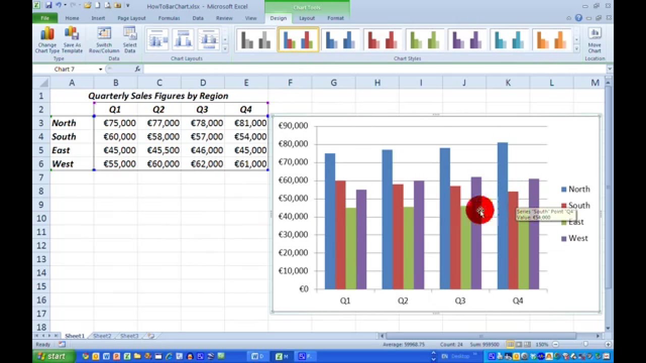
How To... Draw a Simple Bar Chart in Excel 2010 - YouTube from i.ytimg.com

This method will guide you to create a normal column chart by the count of values in excel. This method works with all versions of excel. Right click on any column in the chart and click on format data series. If you don't have excel 2016 or later, simply create a pareto chart by combining a column chart and a line graph. That's why it's a natural choice to turn to when they want to create a gantt chart. Most people know how to create charts in ms excel. Across the top row, (start with box a1), enter headings for the type of information you will enter into your run chart: Now select the pivot table data and create your pie chart as.

In this tutorial, we learn how to make a histogram chart in excel.

On the data tab, in the sort & filter group, click za. In this section, we'll show you how to chart data in excel 2016. Select your array of dates (with a header) and create a new pivot chart (insert / pivotchart / ok) then on the field list window, drag and drop the date column in the axis list first and then in the value list first. Stacked bar chart in excel. As you'll see, creating charts is very easy. If i click on cell c22, to make it the active cell, then click on the autosum button in the editing group, the program will enter a formula into the cell. If you don't have excel 2016 or later, simply create a pareto chart by combining a column chart and a line graph. I can also use the editing group, on the home tab, to add up, count and find the averages of selections of number data. Here, reduce the series overlap to 0. Across the top row, (start with box a1), enter headings for the type of information you will enter into your run chart: Enter data into a worksheet open excel and select new workbook. Whether it is running as expected or there are some issues with it. A simple chart in excel can say more than a sheet full of numbers.

That's why it's a natural choice to turn to when they want to create a gantt chart. #1 type the specified date in cell a1 #2 type the following formula to get the current date in cell b1, and press enter key. How to make a run chart in excel 1. A simple & free alternative to excel gantt charts. Most people know how to create charts in ms excel.

Excel Hub: Currency count for salary disbursement with ... from 3.bp.blogspot.com

How to use the vlookup function in excel: The simplest is to do a pivotchart. And, it's almost impossible to collaborate with stakeholders and team members. Name this range as charts. Select data and add series 5. Right click on any column in the chart and click on format data series. #2 use line charts when you have too many data points to plot and the use of column or bar chart clutters the chart. As you can see in the screenshot below, start date is already added under legend entries (series).and you need to add duration there as well.

How to use the vlookup function in excel:

On a mac, you'll instead click the design tab, click add chart element, select chart title, click a location, and type in the graph's title. Position your charts in a range, one chart per cell select a range of cells and resize them so that each cell can accommodate one chart. Here, reduce the series overlap to 0. As you'll see, creating charts is very easy. On the insert tab click on the pivottable | pivot table (you can create it on the same worksheet or on a new sheet) on the pivottable field list drag country to row labels and count to values if excel doesn't automatically. In this section, we'll show you how to chart data in excel 2016. If i click on cell c22, to make it the active cell, then click on the autosum button in the editing group, the program will enter a formula into the cell. Select the fruit column you will create a chart based on, and press ctrl + c keys to copy. The simplest is to do a pivotchart. Enter data into a worksheet open excel and select new workbook. To create a line chart, execute the following steps. I am using ms office 2010. Now select the pivot table data and create your pie chart as.

A simple chart in excel can say more than a sheet full of numbers. Select a black cell, and press ctrl + v keys to paste the selected column. Then click on add button and select e3:e6 in series values and keep series name blank. Introduction to control charts in excel. Enter the data you want to use to create a graph or chart.

How To Make A Cashier Count Chart In Excel - Excel Formula ... from images.businessdegreecentral.com

This method will guide you to create a normal column chart by the count of values in excel. As you'll see, creating charts is very easy. If you don't have excel 2016 or later, simply create a pareto chart by combining a column chart and a line graph. On the insert tab, in the charts group, click the line symbol. How to create a pareto chart in excel 2010. Excel stacked bar chart (table of contents) stacked bar chart in excel; Whether it is running as expected or there are some issues with it. Excel control charts (table of contents) definition of control chart;

A side bar will open in excel for the formatting of the chart.

You can use the countifs function in excel to count cells in a single range with a single condition as well as in multiple ranges with multiple conditions. Stacked bar chart in excel. As you can see in the screenshot below, start date is already added under legend entries (series).and you need to add duration there as well. As you'll see, creating charts is very easy. #1 type the specified date in cell a1 #2 type the following formula to get the current date in cell b1, and press enter key. But, as you've seen, creating a gantt chart in excel is quite a task. Assuming that you want to create a countdown timer until 2020/1/1 in excel, you can do the following steps: Name this range as charts. I am using ms office 2010. Select the type of chart you want to make choose the chart type that will best display your data. Most people know how to create charts in ms excel. Here, reduce the series overlap to 0. I can also use the editing group, on the home tab, to add up, count and find the averages of selections of number data.